Custom PyTorch model in a zea.Pipeline

This example demonstrates how to embed a custom PyTorch model (defined in code) into a zea.Pipeline using a Lambda operation.

We use the PICMUS ultrasound dataset, perform beamforming, and run a simple torch image processing model (blurring) on the resulting B-mode image.

 

‼️ Important: This notebook is optimized for GPU/TPU. Code execution on a CPU may be very slow.

If you are running in Colab, please enable a hardware accelerator via:

Runtime → Change runtime type → Hardware accelerator → GPU/TPU 🚀.

%%capture
%pip install zea

import os

os.environ["KERAS_BACKEND"] = "torch"

import torch
import torch.nn as nn
import numpy as np
import keras
from IPython.display import display

import zea
from zea.visualize import set_mpl_style
from zea.ops import (
    Pipeline,
    Cast,
    EnvelopeDetect,
    Normalize,
    LogCompress,
    Beamform,
    Lambda,
)

zea: Using backend 'torch'

Let’s set the parameters for the beamforming grid.

grid_size_x = 200
grid_size_z = 300

device = zea.init_device(verbose=False, hide_others=False)
set_mpl_style()

Load a Frame from the PICMUS Dataset

We use the zea loader to load a single frame of raw RF data from the PICMUS dataset, along with scan and probe parameters.

# Load a single frame of raw RF data from PICMUS
path = "hf://zeahub/picmus/database/experiments/contrast_speckle/contrast_speckle_expe_dataset_iq/contrast_speckle_expe_dataset_iq.hdf5"
with zea.File(path, mode="r") as file:
    data = file.data.raw_data[:]
    parameters = file.load_parameters()

zlims = (0, 0.06)
xlims = (-0.019, 0.019)
dynamic_range = (-50, 0)

parameters.zlims = zlims
parameters.xlims = xlims
parameters.grid_size_x = grid_size_x
parameters.grid_size_z = grid_size_z

Build a zea Pipeline for Beamforming and Image Formation

Let’s build an example ultrasound image formation pipeline. We use a PatchedGrid pipeline for memory-efficient beamforming, followed by envelope detection, normalization, and log compression. JIT compilation is supported on the "torch" backend through torch.compile, just as it is on "jax" and "tensorflow". We pass jit_options=None here to skip the one-off compilation warm-up, which dominates the runtime of a single-frame example like this one; for repeated calls leave it at its "ops" default.

pipeline = Pipeline(
    operations=[
        Cast(dtype="float32"),
        Beamform(
            beamformer="delay_and_sum",
            num_patches=100,
            jit_options=None,
        ),
        EnvelopeDetect(),
        Normalize(),
        LogCompress(),
    ],
    with_batch_dim=True,
    device=device,
    jit_options=None,
)

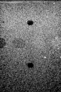
We prepare the parameters for the pipeline and run it to obtain a B-mode image.

inputs = pipeline.prepare_parameters(parameters, dynamic_range=dynamic_range, device=device)

with zea.device(device):
    inputs[pipeline.key] = keras.ops.convert_to_tensor(data)
    outputs = pipeline(**inputs)
    bmode = outputs[pipeline.output_key]

    bmode_img = zea.display.to_8bit(bmode[0], dynamic_range=dynamic_range)
    display(bmode_img)

zea: WARNING width/grid_size_x = 0.0001900 > wavelength/2 = 0.0001478. Consider increasing grid_size_x to 258 or more, or unsetting it to size the grid automatically.
zea: WARNING depth/grid_size_z = 0.0002000 > wavelength/2 = 0.0001478. Consider increasing grid_size_z to 406 or more, or unsetting it to size the grid automatically.

Embedding a custom PyTorch model

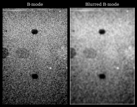
We define a simple torch model that applies a Gaussian blur using a convolutional layer with fixed weights.

class TorchGaussianBlur(nn.Module):
    def __init__(self, kernel_size=7, sigma=2.0):
        super().__init__()
        self.kernel_size = kernel_size
        self.sigma = sigma
        self.padding = kernel_size // 2

        # Create Gaussian kernel
        ax = np.arange(-self.padding, self.padding + 1)
        xx, yy = np.meshgrid(ax, ax)
        kernel = np.exp(-(xx**2 + yy**2) / (2 * sigma**2))
        kernel = kernel / np.sum(kernel)
        kernel = kernel.astype(np.float32)
        kernel = kernel[None, None, :, :]  # shape (1, 1, k, k)
        self.register_buffer("weight", torch.from_numpy(kernel))

    def forward(self, x):
        C = x.shape[1]
        weight = self.weight.repeat(C, 1, 1, 1)
        return torch.nn.functional.conv2d(x, weight, padding=self.padding, groups=C)

To embed this model in the zea pipeline, we use a Lambda operation that applies the model to the B-mode image. We first need to wrap the model call in a simple function that takes the image as input and returns the processed image.

torch_blur_model = TorchGaussianBlur(kernel_size=7, sigma=2.0)
torch_blur_model.to(device)
torch_blur_model.eval()


def torch_blur_inference(image):
    """Simple example inference function for the torch model."""
    image = image.to(torch_blur_model.weight.device)
    with torch.no_grad():
        # (H, W) -> (1, 1, H, W)
        out = torch_blur_model(image[None, None])
    return out[0, 0]  # (1, 1, H, W) -> (H, W)

Add a Lambda Operation to an existing Pipeline

We add a Lambda operation to the pipeline to run the torch blurring model on the B-mode image.

blurring_pipeline = Pipeline(
    operations=[
        pipeline,
        Lambda(func=torch_blur_inference, key=pipeline.output_key, output_key="blurred"),
    ],
    with_batch_dim=True,
    jit_options=None,
    device=device,
)

Run the pipeline and visualize the blurred image.

result = blurring_pipeline(**inputs)
blurred = result["blurred"]

with zea.device("cpu"):
    blurred = zea.display.to_8bit(
        blurred[0],
        dynamic_range=dynamic_range,
        pillow=False,
    )
    bmode_img = zea.display.to_8bit(
        bmode[0],
        dynamic_range=dynamic_range,
        pillow=False,
    )
    fig, _ = zea.visualize.plot_image_grid(
        [bmode_img, blurred],
        titles=["B-mode", "Blurred B-mode"],
        cmap="gray",
        figsize=(10, 5),
    )