Working with the zea data format

In this tutorial notebook we will show how to load a zea data file and how to access the data stored in it. There are three common ways to load a zea data file:

1. Loading data from single file with zea.File

2. Loading data from a group of files with zea.Dataset

3. Loading data in batches with dataloading utilities with zea.Dataloader

   

‼️ Important: This notebook is optimized for GPU/TPU. Code execution on a CPU may be very slow.

If you are running in Colab, please enable a hardware accelerator via:

Runtime → Change runtime type → Hardware accelerator → GPU/TPU 🚀.

%%capture
%pip install zea

config_picmus_iq = "hf://zeahub/configs/config_picmus_iq.yaml"

import os

os.environ["KERAS_BACKEND"] = "jax"

import keras
import matplotlib.pyplot as plt

import zea
from zea.visualize import set_mpl_style

zea: Using backend 'jax'

We will work with the GPU if available, and initialize using init_device to pick the best available device. Also, (optionally), we will set the matplotlib style for plotting.

zea.init_device(verbose=False)
set_mpl_style()

Loading a file with zea.File

The zea data format works with HDF5 files. We can open a zea data file using the h5py package and have a look at the contents using the zea.File.summary() function. You can see that every dataset element contains a corresponding description and unit. Note that we now pass a url to a Hugging Face dataset, but you can also use a local file path to a zea data file. Here we will use an example from the PICMUS dataset, converted to zea format and hosted on the Hugging Face Hub.

Tip: You can also use the HDFView tool to view the contents of the zea data file without having to run any code. Or if you use VS Code, you can install the HDF5 extension to view the contents of the file.

You can extract data and acquisition parameters (which are stored together with the data in the zea data file) as follows:

file_path = "hf://zeahub/picmus/database/experiments/contrast_speckle/contrast_speckle_expe_dataset_iq/contrast_speckle_expe_dataset_iq.hdf5"

# we'll only load the first frame and the first 3 transmit events here
frame_idx = 0
transmit_idx = slice(0, 3)

with zea.File(file_path, mode="r") as file:
    file.summary()
    data = file.data.raw_data[frame_idx, transmit_idx]
    parameters = file.load_parameters()

print("Raw data shape:", data.shape)
print(parameters)

contrast_speckle_expe_dataset_iq.hdf5/
├── description: "PICMUS (Plane-wave Imaging Challenge in Medical UltraSound) dataset converted to zea format. License: The datasets and code provided on PICMUS are free of use. The only request is to refer properly to PICMUS - The Plane Wave Imaging Challenge in Medical UltraSound and quote the proceeding paper.. Citation: H. Liebgott, A. Rodriguez-Molares, F. Cervenansky, J. D'hooge, O. Bernard. "Plane-Wave Imaging Challenge in Medical Ultrasound." 2016 IEEE International Ultrasonics Symposium (IUS), Tours, France, 2016, pp. 1-4. https://doi.org/10.1109/ULTSYM.2016.7728908"
├── zea_version: "0.1.0"
├── metadata/
│   ├── credit: "H. Liebgott, A. Rodriguez-Molares, F. Cervenansky, J. D'hooge, O. Bernard. "Plane-Wave Imaging Challenge in Medical Ultrasound." 2016 IEEE International Ultrasonics Symposium (IUS), Tours, France, 2016, pp. 1-4. https://doi.org/10.1109/ULTSYM.2016.7728908"  Credit or attribution for the dataset.
│   └── subject/
│       └── type: "phantom"
├── metrics/
├── probe/
│   ├── element_height: 0.005  [m]  Height (elevation aperture) of a single transducer element.
│   ├── element_width: 0.00027  [m]  Width of a single transducer element.
│   ├── name: "verasonics_l11_4v"  Probe model name/identifier.
│   ├── probe_bandwidth_percent: 67  [%]  Fractional bandwidth as a percentage.
│   ├── probe_center_frequency: 5133300  [Hz]  Probe nominal centre frequency.
│   ├── probe_geometry (shape=(128, 3), dtype=float32)  [m]  Element positions (x, y, z) per element, shape (n_el, 3).
│   └── type: "linear"  Probe geometry type (linear, phased, curved, ...).
└── tracks/
    └── track_0/
        ├── data/
        │   └── raw_data (shape=(1, 75, 832, 128, 2), dtype=float32)  Raw channel data.
        └── scan/
            ├── azimuth_angles (shape=(75), dtype=float32)  [rad]  Azimuthal angles of transmit beams.
            ├── center_frequency: 5208000  [Hz]  Center frequency of the transmit pulse.
            ├── demodulation_frequency: 5208000  [Hz]  Demodulation frequency.
            ├── focus_distances (shape=(75), dtype=float32)  [m]  Transmit focus distances.
            ├── initial_times (shape=(75), dtype=float32)  [s]  A/D converter start times per transmit.
            ├── polar_angles (shape=(75), dtype=float32)  [rad]  Polar angles of transmit beams.
            ├── sampling_frequency: 5208000  [Hz]  Sampling frequency.
            ├── sound_speed: 1540  [m/s]  Speed of sound.
            ├── t0_delays (shape=(75, 128), dtype=float32)  [s]  Transmit delays per element.
            ├── transmit_origins (shape=(75, 3), dtype=float32)  [m]  Transmit beam origins (x, y, z).
            └── tx_apodizations (shape=(75, 128), dtype=float32)  Transmit apodization per element.
Raw data shape: (3, 832, 128, 2)
Parameters(
    probe_center_frequency=np.float32(5.1333e+06),
    probe_bandwidth_percent=np.float32(67.0),
    probe_geometry=array(float32 (128, 3)),
    element_width=np.float32(0.00027),
    element_height=np.float32(0.005),
    sampling_frequency=5.208 MHz,
    center_frequency=5.208 MHz,
    demodulation_frequency=5.208 MHz,
    initial_times=array(float32 (75,)),
    t0_delays=array(float32 (75, 128)),
    tx_apodizations=array(float32 (75, 128)),
    focus_distances=array(float32 (75,)),
    transmit_origins=array(float32 (75, 3)),
    polar_angles=array(float32 (75,)),
    azimuth_angles=array(float32 (75,)),
    sound_speed=np.float32(1540.0),
    n_ax=832,
    n_el=np.int32(128),
    n_tx=np.int32(75),
    pixels_per_wavelength=np.int32(4),
    pfield_kwargs={},
    apply_lens_correction=False,
    enable_scanline=False,
    focal_region_length=np.float32(0.0),
    grid_type='cartesian',
    selected_transmits=[0, 1, 2, 3, ..., 73, 74] (len=75),
    attenuation_coef=np.float32(0.0),
    f_number=1.0,
    distance_to_apex=np.float32(0.0)
)

Loading data with zea.Dataset

We can also load and manage a group of files (i.e. a dataset) using the zea.Dataset class. Instead of a path to a single file, we can pass a list of file paths or a directory containing multiple zea data files. The zea.Dataset class will automatically load the files and allow you to access the data in a similar way as with zea.File. Note that you can pass zea.Dataset(..., lazy=True) to only load the data once a file is accessed, which can be useful when working with large datasets.

dataset_path = "hf://zeahub/picmus/database/experiments"

with zea.Dataset(dataset_path, lazy=True) as dataset:
    print(dataset)

    for file in dataset:
        print(file)

Dataset with 4 files
<File "contrast_speckle_expe_dataset_iq.hdf5" (mode r, 1 track)>

<File "contrast_speckle_expe_dataset_rf.hdf5" (mode r, 1 track)>

<File "resolution_distorsion_expe_dataset_iq.hdf5" (mode r, 1 track)>

<File "resolution_distorsion_expe_dataset_rf.hdf5" (mode r, 1 track)>

Loading data with Dataloader

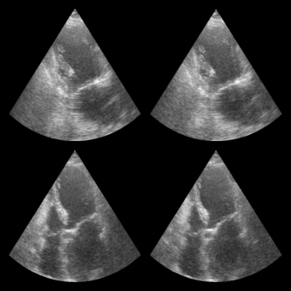
In machine and deep learning workflows, we often want more features like batching, shuffling, and parallel data loading. The zea.Dataloader class provides a convenient way to create a high-performance data loader from a zea dataset. It is built on Grain and does not require TensorFlow. This dataloader is particularly useful for training models. Consistency of shape is preferred, which is not the case for PICMUS. Therefore in this example we will use a small part of the CAMUS dataset.

dataset_path = "hf://zeahub/camus-sample/val"
dataloader = zea.Dataloader(
    dataset_path,
    key="data/image/values",
    batch_size=4,
    shuffle=True,
    clip_image_range=[-60, 0],
    image_range=[-60, 0],
    normalization_range=[0, 1],
    image_size=(256, 256),
    resize_type="resize",  # or "center_crop or "random_crop"
    seed=4,
)

for batch in dataloader:
    print("Batch shape:", batch.shape)
    break  # Just show the first batch

fig, _ = zea.visualize.plot_image_grid(batch)

zea: Searching /root/.cache/zea/huggingface/datasets/datasets--zeahub--camus-sample/snapshots/a41a18873d22100d756186b5d402184b62f3b626/val for ['.hdf5', '.h5'] files...
zea: Running _find_h5_file_shapes and caching the result to /root/.cache/zea/cached_funcs/_find_h5_file_shapes_a26286e42dc8cd2a6e1234c7911a8201.pkl.
Batch shape: (4, 256, 256, 1)

Processing an example

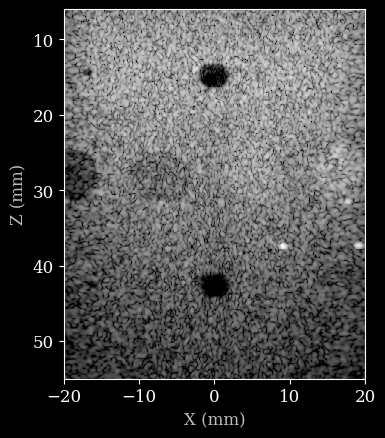
We will now use one of the zea data files to demonstrate how to process it. A full example can be found in the zea_pipeline_example notebook. Here we will just show a simple example for completeness. We will start by loading a config file, that contains all the required information to initiate a processing pipeline.

config = zea.Config.from_path(config_picmus_iq, revision="v0.1.0a1")

Now we can load the zea data file, extract data and parameters, and then process the data using the pipeline defined by the config file.

with zea.File(file_path, mode="r") as file:
    parameters = file.load_parameters()
    # we use config here to overwrite some of the scan parameters
    parameters.update(**config.parameters)
    data = file.data.raw_data[:]

pipeline = zea.Pipeline.from_config(config)
inputs = pipeline.prepare_parameters(parameters)

images = pipeline(data=data, **inputs)["data"]
images = keras.ops.convert_to_numpy(images)

Finally we can plot the result.

image = zea.display.to_8bit(images[0], dynamic_range=(-50, 0))
plt.figure()
# Convert xlims and zlims from meters to millimeters for display
xlims_mm = [v * 1e3 for v in parameters.xlims]
zlims_mm = [v * 1e3 for v in parameters.zlims]
plt.imshow(image, cmap="gray", extent=[xlims_mm[0], xlims_mm[1], zlims_mm[1], zlims_mm[0]])
plt.xlabel("X (mm)")
plt.ylabel("Z (mm)")

Text(0, 0.5, 'Z (mm)')