REFoCUS: Synthetic Aperture Recovery for Ultrasound Imaging
In this notebook, we demonstrate how to use the Refocus operation to decode plane-wave transmit data into synthetic aperture (SA) data, and how it affects the resulting B-mode image quality.
REFoCUS works by inverting the transmit encoding model in the frequency domain, effectively recovering a full-matrix capture (multistatic) dataset from a conventional plane-wave or focused transmit sequence. This can improve lateral resolution and contrast compared to standard delay-and-sum beamforming.
References
Bottenus, N. (2018). Recovery of the complete data set from focused transmit beams. IEEE Transactions on Ultrasonics, Ferroelectrics, and Frequency Control, 65(1), 30–38. https://doi.org/10.1109/TUFFC.2017.2773495
Ali, R., Dahl, J., & Bottenus, N. (2019). Extending Retrospective Encoding for Robust Recovery of the Multistatic Dataset. IEEE TUFFC, 67(5), 943–956.
Reference implementation: https://github.com/nbottenus/REFoCUS
![]()
‼️ Important: This notebook is optimized for GPU/TPU. Code execution on a CPU may be very slow.
If you are running in Colab, please enable a hardware accelerator via:
Runtime → Change runtime type → Hardware accelerator → GPU/TPU 🚀.
[1]:
%%capture
%pip install zea
[2]:
import os

os.environ["KERAS_BACKEND"] = "jax"
os.environ["ZEA_DISABLE_CACHE"] = "1"
os.environ["ZEA_LOG_LEVEL"] = "INFO"
We’ll import all necessary libraries and modules, including the Refocus and Pipeline classes.
[3]:
import matplotlib.pyplot as plt

import zea
from zea.display import to_8bit
from zea.ops import (
    Pipeline,
    Cast,
    Refocus,
    ApplyWindow,
    Demodulate,
    Beamform,
    EnvelopeDetect,
    Normalize,
    LogCompress,
)
from zea.visualize import set_mpl_style
zea: Using backend 'jax'
We will work with the GPU if available, and initialize using init_device to pick the best available device. We also set the matplotlib style for consistent plot styling.
[4]:
zea.init_device(verbose=False)
set_mpl_style()
Loading data
We’ll load a real RF dataset from the PICMUS challenge. This is a contrast-speckle phantom acquired with a plane-wave sequence using 75 transmit angles.
[5]:
num_transmits = 75
grid_size_x = None
grid_size_z = None
[6]:
path = "hf://zeahub/picmus/database/experiments/contrast_speckle/contrast_speckle_expe_dataset_rf/contrast_speckle_expe_dataset_rf.hdf5"

with zea.File(path, mode="r", revision="v0.1.0") as file:
    data = file.data.raw_data[0]
    parameters = file.load_parameters()

data = data[None, ...]

parameters.set_transmits(num_transmits)
data = data[:, parameters.selected_transmits]

if grid_size_x is not None:
    parameters.grid_size_x = grid_size_x
if grid_size_z is not None:
    parameters.grid_size_z = grid_size_z

print(
    f"n_frames: {data.shape[0]}\n"
    f"n_tx:     {data.shape[1]}\n"
    f"n_ax:     {data.shape[2]}\n"
    f"n_el:     {data.shape[3]}\n"
    f"n_ch:     {data.shape[4]}"
)
n_frames: 1
n_tx:     75
n_ax:     3328
n_el:     128
n_ch:     1
Since we’ll be displaying B-mode images several times, let’s define a small helper function.
[7]:
def plot_bmode(ax, image, parameters, title="", dynamic_range=(-60, 0)):
    """Display a B-mode image with physical axis labels."""
    xlims_mm = [v * 1e3 for v in parameters.xlims]
    zlims_mm = [v * 1e3 for v in parameters.zlims]
    ax.imshow(
        to_8bit(image, dynamic_range=dynamic_range),
        cmap="gray",
        extent=[xlims_mm[0], xlims_mm[1], zlims_mm[1], zlims_mm[0]],
        aspect="equal",
    )
    ax.set_xlabel("x (mm)")
    ax.set_ylabel("z (mm)")
    ax.set_title(title)
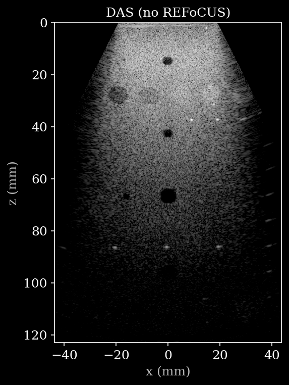
Baseline: standard DAS pipeline
First, let’s run the default Pipeline without REFoCUS to establish a baseline B-mode image using standard delay-and-sum (DAS) beamforming.
[8]:
pipeline = Pipeline(
    [
        Cast(dtype="float32"),
        Demodulate(),
        Beamform(
            beamformer="delay_and_sum",
            num_patches=200,
            enable_pfield=False,
        ),
        EnvelopeDetect(),
        Normalize(),
        LogCompress(),
    ]
)
inputs = pipeline.prepare_parameters(parameters)

inputs[pipeline.key] = data
outputs = pipeline(**inputs)
image_das = outputs[pipeline.output_key]

fig, ax = plt.subplots(figsize=(4, 6))
plot_bmode(ax, image_das[0], parameters, title="DAS (no REFoCUS)")
plt.tight_layout()
plt.savefig("refocus_bmode_das.png", dpi=150, bbox_inches="tight")
plt.close()
REFoCUS pre-processing
The Refocus operation is prepended to any existing pipeline. It decodes the plane-wave data into a synthetic aperture dataset, which is then passed to the downstream beamformer as if it came from individual element firings.
It supports four inversion methods:
Method |
Description |
|---|---|
|
Matched-filter pseudo-inverse. Fast and parameter-free. With |
|
Tikhonov-regularized least-squares inverse. |
|
Truncated SVD. Singular values below |
|
Regularized SVD, similar to Tikhonov but in the SVD domain. |
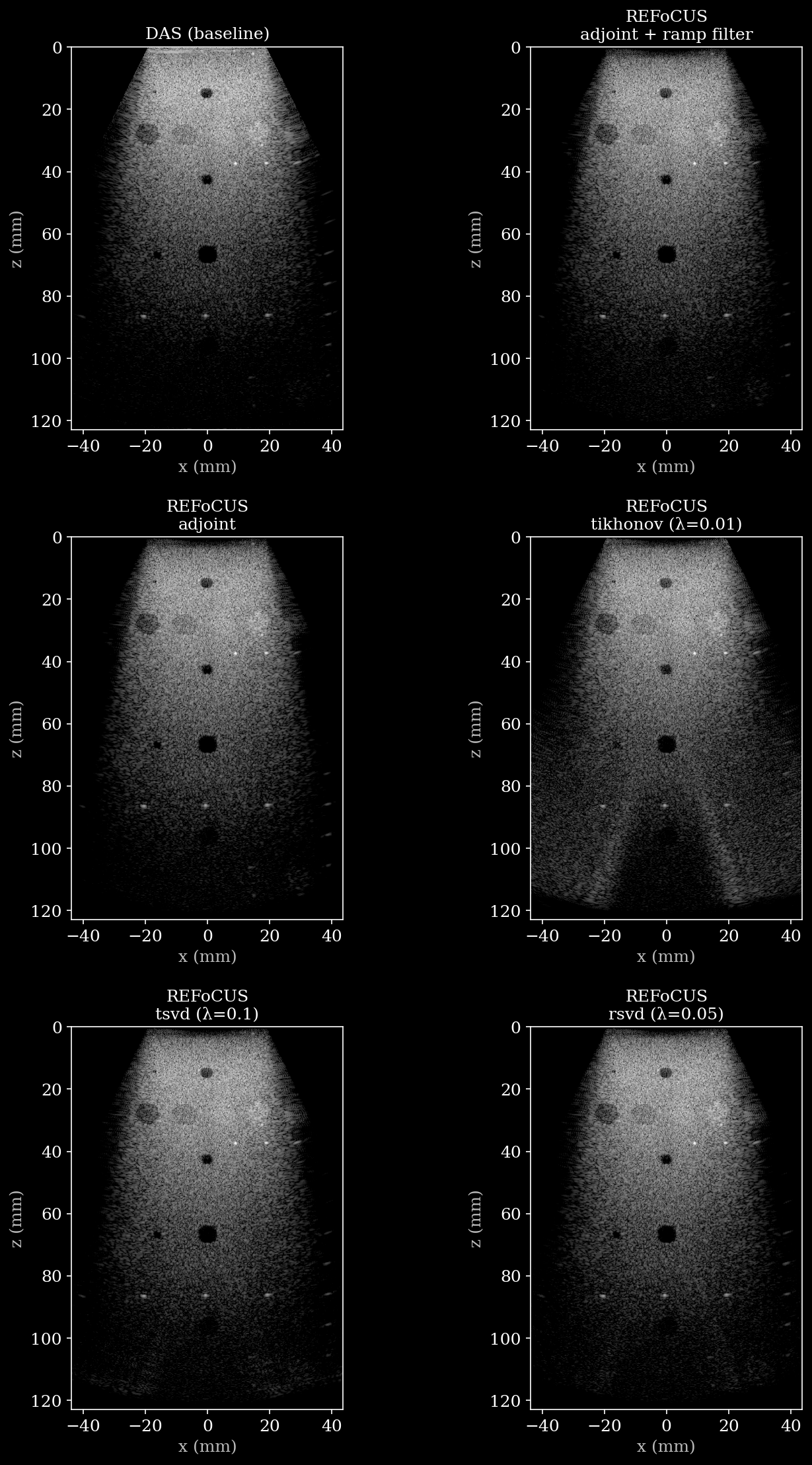
Below we run all four methods and compare the resulting images side-by-side against the baseline.
[9]:
refocus_configs = [
    {"method": "adjoint", "param": None, "label": "adjoint + ramp filter"},
    {"method": "adjoint", "param": 0, "label": "adjoint"},
    {"method": "tikhonov", "param": 0.01, "label": "tikhonov (λ=0.01)"},
    {"method": "tsvd", "param": 0.1, "label": "tsvd (λ=0.1)"},
    {"method": "rsvd", "param": 0.05, "label": "rsvd (λ=0.05)"},
]

n_cols = 2
n_rows = (len(refocus_configs) + 2) // n_cols
fig, axes = plt.subplots(n_rows, n_cols, figsize=(10, n_rows * 5))
axes = axes.flatten()

# Baseline (no REFoCUS)
plot_bmode(axes[0], image_das[0], parameters, title="DAS (baseline)")

for i, cfg in enumerate(refocus_configs):
    pipeline = Pipeline(
        [
            Cast(dtype="float32"),
            ApplyWindow(size=64, start=64),
            Refocus(method=cfg["method"], param=cfg["param"], jit_compile=False),
            Demodulate(),
            Beamform(
                beamformer="delay_and_sum",
                num_patches=200,
                enable_pfield=False,
            ),
            EnvelopeDetect(),
            Normalize(),
            LogCompress(),
        ]
    )

    inputs = pipeline.prepare_parameters(parameters)

    outputs = pipeline(**{pipeline.key: data}, **inputs)
    image = outputs[pipeline.output_key]

    plot_bmode(axes[i + 1], image[0], parameters, title=f"REFoCUS\n{cfg['label']}")

# Hide any unused axes
for ax in axes[len(refocus_configs) + 1 :]:
    ax.set_visible(False)

plt.tight_layout()
plt.savefig("refocus_example.png", dpi=150, bbox_inches="tight")
plt.close()